Applying Detrend Data to CCDs
Setting an astrometry file
You have prepared detrend data. Next reduction is applying detrend data to each [visit, ccd] of object data. It will be done by reduceFrames.py in HSC pipeline. During the process of reduceFrames.py, magnitude zero-points and WCS are also determined for the next process of Mosaicing. Thus, we need to set an astrometry file before performing reduceFrames.py.
# Setting a catalog file for the astrometry
# If you use SDSS catalog,
setup astrometry_net_data sdss-dr9-fink-v5b
# If you use Pan-STARRS catalog,
setup astrometry_net_data ps1_pv3_3pi_20170110-and
Note
If you need to prepare an original catalog file, such as for NB reduction, please refer to How to make an astrometry file.
Warning
You must set an astrometry file, when you login your machine!!!
Applying detrend data:performing reduceFrames.py
After setting an astrometry file, next process is to perform reduceFrames.py. Detrending, calibration, detection, and measurement are performed in reduceFrames.py.
Detrending includes overscan subtraction, bias and dark subtraction, flatfielding, and fringe subtraction. Satulated or bad pixels are masked. After bias subtraction, linearity, crosstalk, and brighter-fatter effect are corrected.
After detrending, calibration starts. The sky background is subtracted using grids of 128 pixels, and then the objects for calibration are detected. PSF of detected objects are measured and photometric zero-points are estimated. Based on this PSF information, cosmic rays are detected and interpolated. The sky background is subtracted again with object masks. After that, detected objects are matched and compared with catalog sources. The WCS and photometric zero-points are determined in each CCDs.
Then the objects are detected and measured. Deblending is executed during detection. Position, shape, and various flux are measured and flags are attached corresponding to pixel masks or events in measurment.
Finally the WCS is fitted across the entire focal plane. The WCS includes the correction for the optical distortion and the images are not warped in this processing.
You can perform reduceFrames.py with a batch process (see batch process ). The reduceFrames.py takes a long time depending on machine environments. Let’s do different work while waiting the reduction.
# Applying detrend data
reduceFrames.py $home/hsc --calib=$home/hsc/CALIB --rerun=dith_16h_test --id filter=HSC-I visit=902798..902808:2 --config processCcd.isr.doFringe=False
reduceFrames.py $home/hsc --calib=$home/hsc/CALIB --rerun=dith_16h_test --id filter=HSC-G visit=903160..903168:2 --config processCcd.isr.doFringe=False

# If you need postISR data (after bias and dark subtraction, flatfielding, and some device-specific process),
reduceFrames.py $home/hsc --calib=$home/hsc/CALIB --rerun=dith_16h_test --id filter=HSC-I visit=902798..902808:2 --config processCcd.isr.doFringe=False processCcd.isr.doWrite=True

# Usage:
#   reduceFrames.py <a directory for data reduction> --calib=<a directory for detrend data> --rerun=<rerun name> --id filter=<filter name> visit=<visit ID of object data> --config <optional parameters>
#
# Parameters:
#   --rerun :Rerun name. You need create new rerun.
#   --id    :Specifying object data.
#             In an example, we set filer name and visit name.
#             Because we have two filters of I-band and G-band, we perform reduceFrame.py for each filter.
#   --config:Specifying additional parameters.
#             We set no use of Fringe data in above example.
Warning
In case of narrow-band filter NB387 and NB515, please refer to here for reduceFrames.py execution.
Once reduceFrames.py is completed, many data is found in $home/hsc/rerun/[rerun]. We introduce each data by reduceFrames.py.
Corrected data and its thumbnails are produced in $home/hsc/rerun/[rerun]/[pointing]/[filter]/corr/ and $home/hsc/rerun/[rerun]/[pointing]/[filter]/thumbs/, respectively. The postISR data are created in $home/hsc/rerun/[rerun]/[pointing]/[filter]/output/postISR
- Correced data (sky background subtracted) :CORR-[visit]-[ccd].fits ( ref:※ <maskedcorr> )
- Sky backgdoun data which is used sky subtraction:BKGD-[visit]-[ccd].fits
- A results of removing overscan :oss-[visit]-[ccd].png
- A result of flattened by Flat data :flattened-[visit]-[ccd].png

Fig 1: Products of reduceFrames.py. Object raw data, overscan removed object data, Flat corrected object data, sky background data, and sky subtracted corrected data are shown from left to right.
Catalogs and all data relating to magnitude zero-points and WCS estimates are in $home/hsc/rerun/[rerun]/[pointing]/[filter]/output/.
- Relatively bright source catalog for the first rough estimates of magnitude zero-points and WCS: ICSRC-[visit]-[ccd].fits
- Source match lists for the first rough estimates of magnitude zero-points and WC : MATCH-[visit]-[ccd].fits
- Column file of MATCH-[visit]-[ccd].fits : ML-[visit]-[ccd].fits
- Source catalog for the second estimates of magnitude zero-points and WCS : SRC-[visit]-[ccd].fits
- Source match lists for the second estimates of magnitude zero-points and WC : SRCMATCH-[visit]-[ccd].fits
- Column file of SRCMATCH-[visit]-[ccd].fits : SRCML-[visit]-[ccd].fits
Contents of MATCH- and ML- fils are basically the same. The difference is
source ID. The source ID of MATCH- can be only referred in HSC pipeline, but
the one of ML- can be used with other software. These catalogs produced in
HSC pipeline are .fits style, and are looked into by
Fv and
TABLES/STSDAS/IRAF .

Fig2: Contents in SRC-.fits using Fv (Left), and contents in ICSRC-.fits by TABLES/STSDAS/IRAF (right).
In this document, we use pyfits supplied with HSC pipeline package to look into catalogs, SRC-[visit]-[ccd].fits. Note that contents of SRC-[visit]-[ccd].fits is listing in Contents of SRC-[visit]-[ccd].fits generated after reduceFrames.py.
# Calling modules
import pyfits
import lsst.afw.display.ds9 as ds9
import lsst.afw.image as afwImage

# Displaying CORR-[visit]-[ccd].fits in ds9
im = afwImage.ImageF("~/hsc/rerun/dith_16h_test/00532/HSC-I/corr/CORR-0902798-059.fits")
ds9.mtv(im)

# Calling up information in SRC-[visit]-[ccd].fits with pyfits
cat = pyfits.open("~/hsc/rerun/dith_16h_test/00532/HSC-I/output/SRC-0902798-059.fits")

# Looking into contents of catalog and its data types
cat[1].data

        # Output
        # ...
        # dtype=[('flags', 'u1', (11,)), ('id', '>i8'), ('coord', '>f8', (2,)), ..., ('centroid_sdss', '>f8', (2,))

cat[1].data['centroid_sdss']

        # Output
        # array([[ 20058.,  19905.],
        #       [ 20126.,  19910.],
        #       [ 20491.,  19907.],
        #       ...,
        #       [ 23760.,  24088.],
        #       [ 23830.,  24054.],
        #       [ 23819.,  24060.]])


# Calling up coordinates of detected objects
xy = cat[1].data["centroid_sdss"]

# Displaying detected objects on ds9
for x, y in xy:
        ds9.dot("o", x, y, size=30)
Note
You can find the usage of pyfits and afw supplied in HSC pipeline in $AFW_DIR/doc/html/index.html.
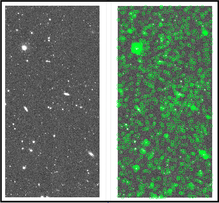
Fig 3: CORR-[visit]-[ccd].fits and sources in SRC-[visit]-[ccd].fits are shown from left to right.
Appendix 1: Evaluations for each [visit, ccd]
You can skip following appendix if you reduce data as soon as possible.
Not only applying detrend data but also evaluation tests for each [visit, ccd] are done by reduceFrames.py. Results of evaluation tests are output in $home/hsc/rerun/[rerun]/[pointing]/[filter]/qa .
Seeing
- A histogram of magnitude of stars used for seeing estimates:magHist-[visit]-[ccd].png
- Intermediate data of seeing estimates :seeingRough-[visit]-[ccd].png
- Results of seeing estimates :seeingRobust-[visit]-[ccd].png

Fig 4: Thumbnails of magHist-, seeingRough- and seeingRobust- are presenting in order from left to right.
- PSF
- A catalog used for PSF estimates :seeingMap-[visit]-[ccd].txt
- Positions and FWHM of stars used for PSF estimates :seeingMap-[visit]-[ccd].png
- A catalog of stars in each grid :seeingGrid-[visit]-[ccd].txt
- The mean FWHM of stars in each grid :fwhmGrid-[visit]-[ccd].png
- The mean FWHM of stars (values) in each grid :fwhmGrid-[visit]-[ccd].fits
- Sizes and positions of stars used for PSF estimates :ellipseMap-[visit]-[ccd].png
- the mean ellipticity of stars in each grid :ellipseGrid-[visit]-[ccd].png
- Positions and ellipticity of stars used for PSF estimates:ellipticityMap-[visit]-[ccd].png
- The mean ellipticity of stars in each grid :ellipticityGrid-[visit]-[ccd].png
- The mean ellipticity of stars (values) in each grid :ellipticityGrid-[visit]-[ccd].fits
- Elongations and ellipticity of stars in each grid :ellPaGrid-[visit]-[ccd].fits
- Stacked images of stars in each grid :psfSrcGrid-[visit]-[ccd].fits
- Stacked images of stars in each grid (contour) :psfSrcGrid-[visit]-[ccd].png
- A PSF model of each grid :psfModelGrid-[visit]-[ccd].fits
- A PSF model of each grid (contour) :psfModelGrid-[visit]-[ccd].png
Note
One grid size is defined as 1024 × 1024 pixels. Megenta circle expresses the mean seeing size of one CCD.
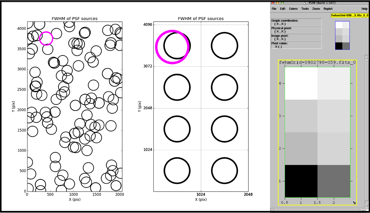
Fig 5: Thumbnails of seeingMap- and fwhmGrid-, and an image of fwhmGrid-.fits are presenting in order from left to right.

Fig 6: Thumbnails of ellipseMap-, ellipseGrid-, ellipticityMap-, ellipticityGrid-, and an image of ellipticityGrid-.fits are presenting in order from left to right.
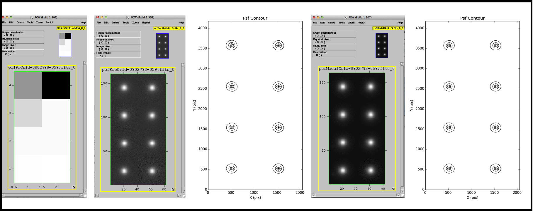
Fig 7: Images of ellPaGrid-fits, psfSrcGrid-fits, a thumbnail of psfSrcGrid-, an image of psfModelGrid-.fits, and a thumbnail of psfModelGrid- are presenting in order from left to right.
Appendix 2: Details of CORR-[visit]-[ccd].fits
CORR-[visit]-[ccd].fits has three layers. Images of corrected data, masked data and variance data are stored in fits[1], [2] and [3], respectively. You can display these images by specifying a layer.
# Displaying corrected data
ds9 CORR-[visit]-[ccd].fits[1]

# Displaying masked data
ds9 CORR-[visit]-[ccd].fits[2]

# Displaying variance data
ds9 CORR-[visit]-[ccd].fits[3]
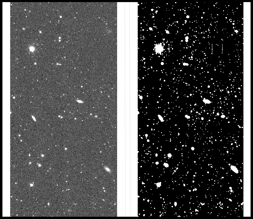
Fig 8: CORR-[visit]-[ccd].fits[1] and CORR-[visit]-[ccd].fits[2] are shown in order from left to right.
Appendix 3: Other products in reduceFrames.py
Other products in reduceFrames.py are icSrc.fits and src.fits in $home/hsc/rerun/[rerun]/schema. They are schema file for source catalogs produced by reduceFrames.py. Although these schema files are automatically produced, they are not used in data reduction.
Additionally, c[104-111].fits is also produced in $home/hsc/rerun/[rerun]/visitim/v[visit]-f[filter]. They are corrected data of focusing CCDs. However, these files are also unusable in subsequent reductions.
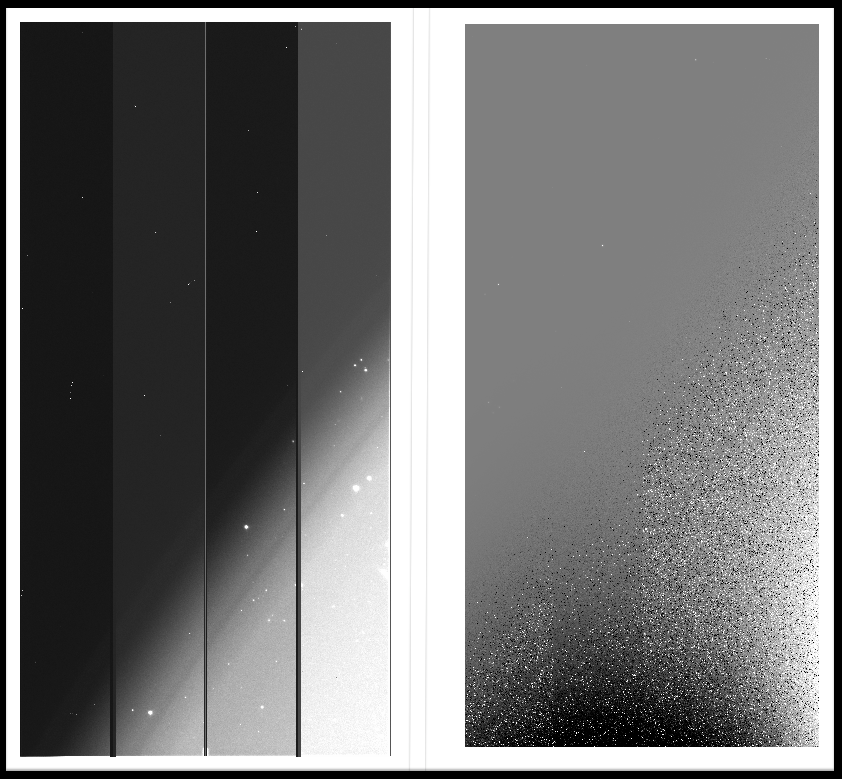
Fig 9: Raw data of a focusing CCD and an image of c[104-111].fits are shown in order from left to right.