Mosaicking
In order to coadd multiple visit images, the tract should be defined and correct wcs and flux scale.
Defining tract
The hscPipe command makeDiscreteSkyMap.py is used to define tract. Based on the coordinates in the header, the tract is determined as a square which covers the whole observed area specified in the command argument. You have to select all visits and filters because the tract definition depends on the selected data. In case of the object observed with two filters, if you execute makeDiscreteSkyMap.py to each filter data, the definition of tract/pateh can be slightly different.
# Assume that a diredctory for reduction is ~/HSC, rerun name test (should be same as previous step), field name test_field (should be checked in registry.sqlite3).
makeDiscreteSkyMap.py ~/HSC --rerun test --id field=test_field

# makeDiscreteSkyMap.py [data reduction directory] --rerun [rerun name] --id [visit, field, filter..]
# Option
#       --id : Specify all data used in tract definition.
You can see the following message when the process succeeds.
makeDiscreteSkyMap INFO: tract 0 has corners (177.676, 57.388), (173.867, 57.388), (173.752, 59.440), (177.790, 59.440) (RA, Dec deg) and 11 x 11 patches

# It means that the tract 0 which has 11x11 patch is determined
Mosaicking
The wcs and flux scale of each visit/CCD data should be corrected to coadd multiple images. It can be done by mosaic.py. This command generates a matched list of reference bright stars from each CCD in a given tract. Then it solves spatially-verying correction terms of relative positions and flux scales on different CCDs/visits.
# A directory for reduction is ~/HSC, and rerun name test
# Execute to each filter
mosaic.py ~/HSC/ --rerun test --id visit=20878..20890:2 tract=0 ccd=0..103

# When you output mosaic validation in ~/HSC/rerun/mosaic_diag,
mosaic.py ~/HSC/ --rerun test --id visit=20878..20890:2 tract=0 ccd=0..103 --diagnostics --diagDir ~/HSC/rerun/mosaic_diag

# mosaic.py [data reduction directory] --rerun [rerun name] --id [visit, field, filter, ccd] tract=[tract]
# Options
#       --id : Specify the object ID. You can also use field and filter. The tract must by selected here.
#       --diagnostics : Add this options if you want to output the results of validation.
#       --diagDir : Specify a output directory for validation.
Note
Depending on the machine enviroument, it takes over 30 minutes after the following messages;
Mosaic INFO: Reading catalogs...
Mosaic INFO: Use 1 cores for reading source catalog
After the processing, flux scaling files fcr-[visit]-[ccd].fits and corrected wcs files wcs-[visit]-[ccd].fits are created in ~/HSC/rerun/[rerun]/jointcal-results/[tract].
If you add –diagnostics option, the results described below are output a directory specified at –diagDir.
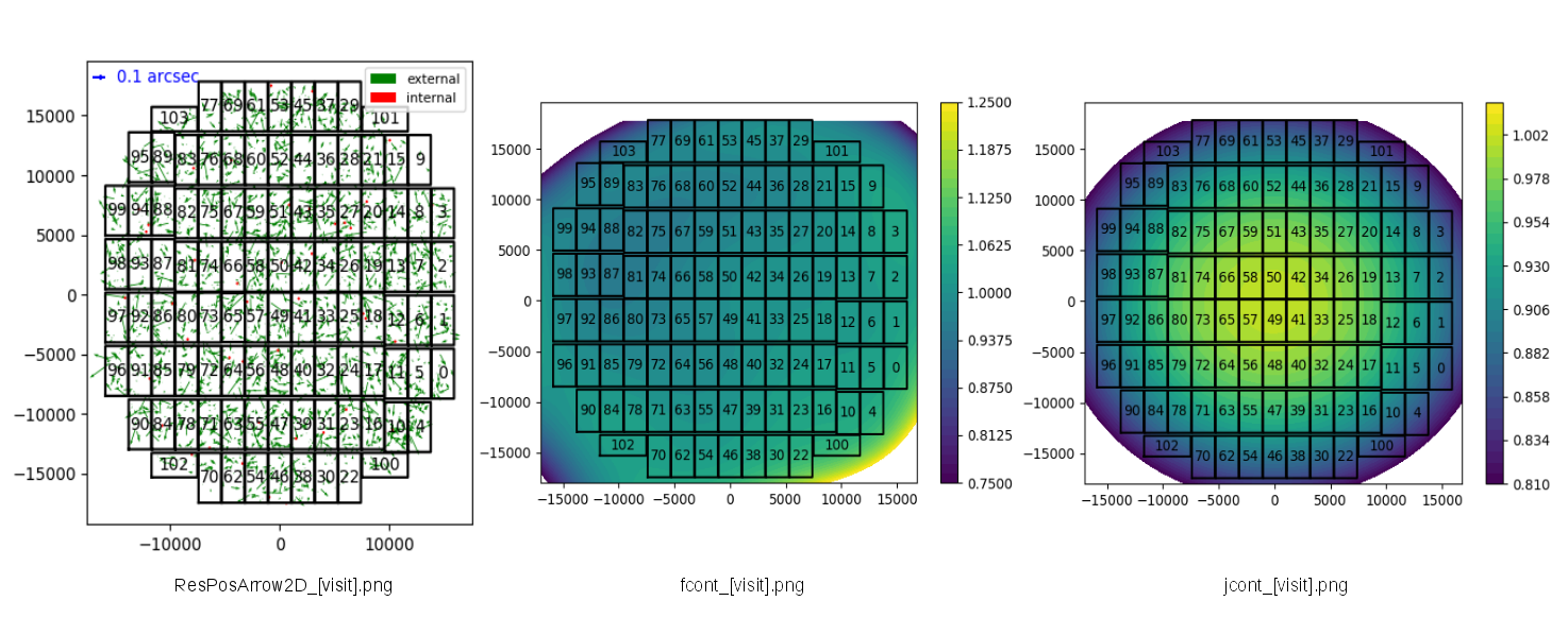
Validation results in each visit
- Positional offsets : ResPosArrow2D_[visit].png
- Residuals of flux to distortion pattern: fcont_[visit].png
- Distortion pattern of reduceFlat : jcont_[visit].png(confirm that distributions is in a concentric fasion)
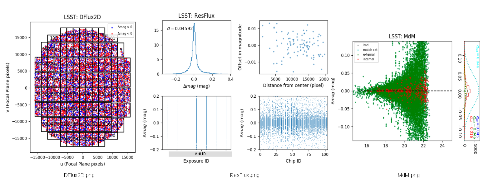
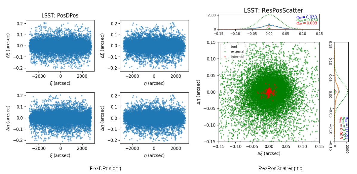
Validation results in all visit
- Deviation from mean flux of each visit: DFlux2D.png
- Residuals of fluxes : ResFlux.png
- Deviation in magnitudes of detected sources (※): MdM.png
- Offsets of WCS : PosDPos.png
- Offsets of WCS : ResPosScatter.png
- Other outputs
- catalog.fits
- ccd.dat
- ccdScale.dat
- coeffs.dat
- dmag.dat
- dpos.dat
(※) Green and red dots denote deviation of catalogs in HSC pipeline from astrometry catalog, and deviation from the mean of all visit in sources which are not in MATCH catalog.
Applying the mosaic solution to each visit/CCD data
Then apply the corrected wcs and flux scale to each visit/CCD data.
Note
If you do not analyze each CCD images and catalogs deeply, you can skip now and perform it at the end of all processing. If you do not need corrected CCD images and catalogs, you don’t have to do this step.
To apply the corrected data to CORR images, calibrateExposure.py is used.
# Applying the solution to the visit/CCD images
# Directory for reduction is ~/HSC, and rerun name test
calibrateExposure.py ~/HSC --rerun test --id field=NGC604 tract=0 ccd=0..103 -j 8

# calibrateExposure.py [data reduction directory] --rerun [rerun name] --id [field, tract, ccd] -j [the number of threads]
# Options
#       --id : In the example, the input data is selected as a combination of field, tract, and ccd. You can also use the combination of visit and ccd.
#       -j : Specify the number of threads.
The calibrated images are generated as ~/HSC/rerun/[rerun]/[pointing]/[filter]/corr/[tract]/CALEXP-[visit]-[ccd].fits
The command calibrateCatalog.py is used to apply to SRC catalogs.
# Applying the solution to catalogs.
# Directory for reduction is ~/HSC, and rerun name test
calibrateCatalog.py ~/HSC --rerun test --id field=NGC604 tract=0 ccd=0..103 --config doApplyCalib=False -j 8

# calibrateCatalog.py [data reduction directory] --rerun [rerun name] --id [field, tract, ccd] -j [the number of threads]
# Options
#       --id : Same as calibrateExposure.py, you can also use the combination of visit and ccd.
#       --config doApplyCalib=False : Add it if you do not calibrate fluxes to magnitudes.
#       -j : Specify the number of threads.
The calibrated catalogs are ~/HSC/rerun/[rerun]/[pointing]/[filter]/output/[tract]/CALSRC-[visit]-[ccd].fits.