Single-visit processing¶

In this page, we describe single-visit processing. We explain Structure of output FITS image at the end of the page.

Single-visit processing, detrending and calibration¶

After preparing data for detrending, next step is the single-visit processing.

The single-visit processing starts with detrending; overscan subtraction, Bias and Dark subtraction, flatfielding, and Fringe subtraction. Then the mask image is generated to indicate bad pixels, crosstalk, and saturated pixels. After Bias subtraction, the linearity and brighter-fatter effect are corrected for each CCD. Next, the calibration part starts. The sky background is subtracted using 128-pixel grids. Bright sources for calibration are detected and their PSFs are measured. The photometric zero-points are estimated by matching them with reference catalog. After that, cosmic ray is removed. Finally sky subtraction is performed on the masked image, and wcs coordinates and photometric zero-point are determined for each CCD. Then the object detection and measurement are performed. During the detection process, objects are deblended. Coordinates, shape, and flux are measured for the detected objects, and mask information or events during measurement are flagged in each pixel. Please see also Bosch et al., 2018, PASJ, 70S, 5B.

These processes are performed with hscPipe command singleFrameDriver.py .

# Assume a directory of reduction is ~/HSC and rerun name test. The object or region name can be the rerun name.
# In case of using local system,
singleFrameDriver.py ~/HSC --calib ~/HSC/CALIB --rerun test --id visit=18214..18220:2^18224..18230:2 --batch-type=smp --cores=8

# If you output the data after detrending,
# For investigation of helpdesk, these data are sometimes required.
singleFrameDriver.py ~/HSC --calib ~/HSC/CALIB --rerun test --id visit=18214..18220:2^18224..18230:2 --config processCcd.isr.doWrite=True --batch-type=smp --cores=8

# singleFrameDriver.py [data reduction directory] --calib [directory of data for detrending] --rerun [rerun name] --id [visit, field, filter..]
# Options
#       --batch-type: The singleFrameDriver.py command can be submitted to batch system.
#       --config processCcd.isr.doBias=False processCcd.isr.doDark=False: If you skip creating Bias and Dark data, add these options.

In typical (the region where stars are not crowded), nearly 2 GB memory would be consumed in 1 process. Please confirm your memory capacity before running the command. It takes about 10 hours to complete processing of 10 shots with 8 cores on HSC data analysis machine for open use (hanaco).

After finishing all processes, you can find corrected CCD images and object catalogs in the follows;

Corrected CCD image (sky background is subtracted) : ~/HSC/rerun/[rerun]/[pointing]/[filter]/corr/CORR-[visit]-[ccd].fits
Sky background image : ~/HSC/rerun/[rerun]/[pointing]/[filter]/corr/BKGD-[visit]-[ccd].fits
Images after overscan subtraction ： ~/HSC/rerun/[rerun]/[pointing]/[filter]/thumbs/oss-[visit]-[ccd].png
Images after flatfielding : ~/HSC/rerun/[rerun]/[pointing]/[filter]/thumbs/flattened-[visit]-[ccd].png
Images after detrending (postISR) : ~/HSC/CALIB/postISRCCD/v[visit]-f[filter]/c[ccd].fits

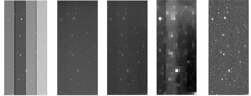
Figure 1：(from left to right) raw data, oss image, flattened image, sky background image, CORR image. Sky background image is adjusted its size because it has a low number of pixels. CORR and sky background image are rotated to align raw data.

The catalogs can be found in /rerun/[rerun]/[pointing]/[filter]/output/;

Catalog of bright sources for calibration : ICSRC-[visit]-[ccd].fits
Catalog of detected sources, output from the final stage of single-visit processing: SRC-[visit]-[ccd].fits
Catalog of detected sources cross-matched with the external reference : SRCMATCH-[visit]-[ccd].fits
Catalog of detected and matched reference sources : SRCMATCHFULL-[visit]-[ccd].fits

These catalogs are in FITS BINTABLE format, so you cannot check the contents with imaging software (e.g., ds9). Fv (Fv FITS Viewer) or STSDAS/TABLES (TABLES) is useful. You can also use PyFITS or IDL.

Figure 2 shows the catalog opened by Fv.

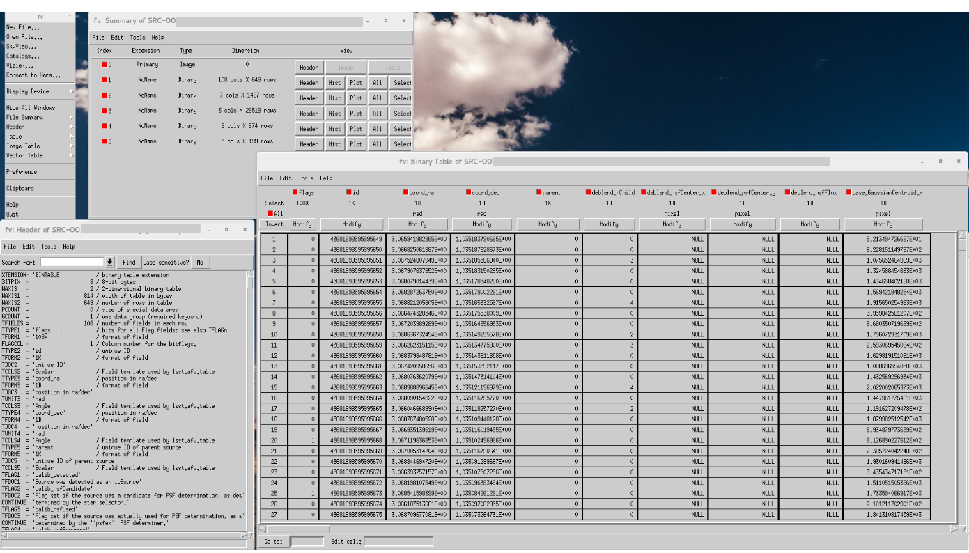
Figure 2：SRC*.fits opened with Fv. The bottom-left panel shows FITS Header, the right shows the main body of the catalog.

There are schema files of catalog in rerun/[rerun]/schema. Note that the column name has been significantly changed from hscPipe4.

In hscPipe, there is “aperture correction” for each photometry algorithm. It is a photometric calibration by using r = 12 pix (4”) diameter circular aperture. For PSF, CModel, or Kron flux, it is corrected as measured by r = 12 pix aperture.

Structure of output FITS image¶

The generated CORR image has 13 HDUs (Header Data Unit) in total;

Primary HDU (HDU0): FITS header
2nd HDU (HDU1): Science image (32bit Float)
3rd HDU (HDU2): Mask image (16bit UInt)
4th HDU (HDU3): Variance
after 5th HDU : Other information (e.g., PSF or aperture correction)

Figure 3 shows science and mask image. You can specify which extension you open by ds9;

# Open science image with ds9
ds9 CORR-[visit]-[ccd].fits
# Or
ds9 CORR-[visit]-[ccd].fits[1]

# Open mask image with ds9
ds9 CORR-[visit]-[ccd].fits[2]

# Open variance image with ds9
ds9 CORR-[visit]-[ccd].fits[3]

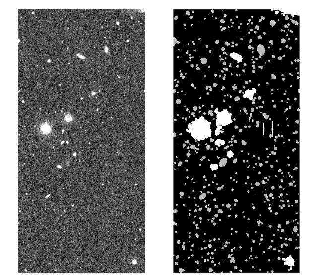
Figure 3：(left) science image and (right) mask image for a CORR*.fits.

You can check the definition of mask bit at the header of a mask image. Fig. 4 shows an example of a mask image header. The mask bit and its event are enclosed by red line. For example, the pixel with value 1024 = 2^10 is flagged as crosstalk because of “HIERARCH MP_CROSSTALK = 10” in the header. For the another pixel, the value 2080 (= 2048 + 32 = 2^11 + 2^5) indicates “Not Deblended” and “Detected”. The relation between bit and event could be changed in each reduction.

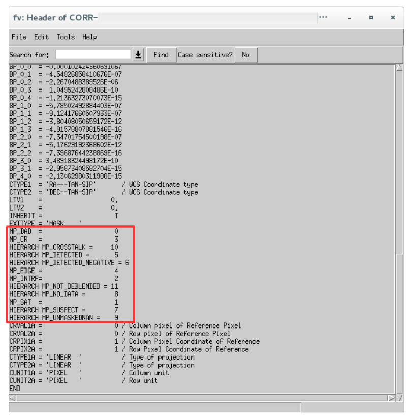
Figure 4: Header of mask image.

We provide the mask viewer to see mask for each event:

https://hsc-gitlab.mtk.nao.ac.jp/sogo.mineo/view-mask/blob/master/view-mask.py

Loading a catalog by PyFITS¶

You can check your catalog and image with pyfits. As an example, we show objects in the SRC catalog on CORR image. The following example uses interactive mode of python. Figure 5 shows the results.

# Setup hscPipe
setup-hscpipe

# Launch python
python

# Import modules
>>> import pyfits
>>> import lsst.afw.display.ds9 as ds9
>>> import lsst.afw.image as afwImage

# Display a CORR file with ds9
>>> corr = afwImage.ImageF("~/HSC/rerun/[rerun]/[pointing]/[filter]/corr/CORR-[visit]-[ccd].fits")
>>> ds9.mtv(corr)

# Loading a catalog
>>> cat = pyfits.open("~/HSC/rerun/[rerun]/[pointing]/[filter]/output/SRC-[visit]-[ccd].fits")
>>> cat[1].data
# Output all data
#       FITS_rec([ ([ ....
#       ...
#       dtype=(numpy.record, [('flags', 'u1', (14,)), ('id', '>i8'), ('coord_ra', '>f8'), ('coord_dec', '>f8'), ('parent', '>i8'),
#       ... ('base_FootprintArea_value', '>i4'), ('base_ClassificationExtendedness_value', '>f8'), ('footprint', '>i4')]))

# Get source coordinates in the catalog
>>> xs = cat[1].data["base_SdssCentroid_x"]
>>> ys = cat[1].data["base_SdssCentroid_y"]

# Plot the sources on the image displayed with ds9
>>> for x,y in zip(xs,ys):
...     ds9.dot("o", x, y, size=30)

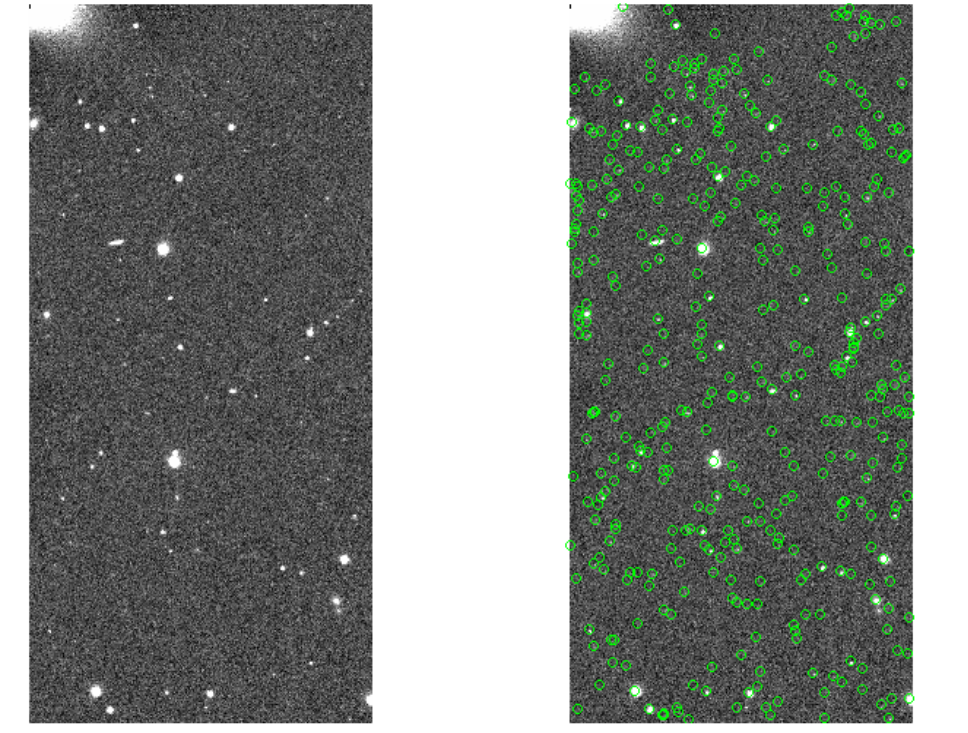
Figure 5：(left) CORR image displayed with ds9. (right) Superpose sources in SRC catalog on the CORR image.

Single-visit processing¶