Pipeline tools
In HSC pipeline, some python-based Pipeline tools are included. You can confirm the image or catalog data. Tools butler and dataRef is useful for searching or loading data, Exposures, MaskedImages, and Images for image processing, and SourceCatalogs for treating coordinates, flus, and size info of objects as a list. In this page, the usage of Pipeline tool is explained briefly.
butler
butler is a tool for searching or loading various type of data (image or catalog). To load the data created in HSC pipeline, get() and dataId is used. For get(), the type of data you want to use (target), [visit, ccd] info of data, and [tract, patch] for coadd data are specified.
# python module calling butler
import lsst.daf.persistence as dafPersist

# Specify rerun directory in which the data you want to use is stored
dataDir = "~/hsc/rerun/dith_16h_test"

# Call butler
butler = dafPersist.Butler(dataDir)

# Specify the target data and searched by butler
#
# CORR-0902798-59.fits
# 'calexp' means CORR-*.fits
dataId = {'visit': 902798, 'ccd': 59}
exp = butler.get('calexp', dataId)
In this example, target = ‘calexp’ is set to load CORR-.fits. Except for this, there are various target is defined like the following list.
| Target | Deta form | Data type |
|---|---|---|
| bias | Bias data | ExposureF |
| dark | Dark data | ExposureF |
| flat | Flat data | ExposureF |
| fringe | Fringe data | ExposureF |
| postISRCCD | post processing data (not created in default setting) | ExposureF |
| calexp | sky subtracted data | ExposureF |
| psf | PSF used in analysis | psf |
| src | object catalog made from detrended data | SourceCatalog |
| wcs, frc | object catalog used in mosaic.py | ExposureI |
| Target | Deta form | Deta type |
|---|---|---|
| deepCoadd_calexp | coadd data | |
| deepCoadd_psf | PSF of coadd image | |
| deepCoadd_src | catalog made from coadd data |
You can check the type of data loaded by butler with dataRef. Then let’s check the information of the data searched by butler above.
# python module which can search HSC pipeline data using butler
import hsc.pipe.base.butler as hscButler

# Loading data by dataRef
dataRef = hscButler.getDataRef(butler, dataId)
ref_exp = dataRef.get('calexp')
ref_exp
        # output:
        # <lsst.afw.image.imageLib.ExposureF; proxy of <Swig Object of type 'boost::shared_ptr< lsst::afw::image::Exposure< float,lsst::afw::image::MaskPixel,lsst::afw::image::VariancePixel > > *' at 0x7f24376a5d50> >

# Loading catalog file having same dataId
ref_cat = dataRef.get('src')
        # output:
        # <lsst.afw.table.tableLib.SourceCatalog; proxy of <Swig Object of type 'lsst::afw::table::SortedCatalogT< lsst::afw::table::SourceRecord > *' at 0x7f24376a5f90> >

# Loading PSF info used in the analysis of same dataId
ref_psf = dataRef.get('psf')
        # output:
        # <lsst.afw.detection.detectionLib.Psf; proxy of <Swig Object of type 'boost::shared_ptr< lsst::afw::detection::Psf > *' at 0x7f24376a5e70> >
Exposures, MaskedImage, Images
Next, 3 Pipeline tools which can display images are introduced. The most simplest one is Images. It can load and show two dimensional images. On the other hand, MaskedImage can process 3 image data (object, mask, and variance image) in CORR-.fits or [patch].fits, and Exposures can read the image which is loaded by MaskedImage and related header info.
The following shows the case that using get() and call MaskedImage, then detrended data subtracted sky background is displayed and saved by matplotlib
# Import python module
# Calling python-based plotter
import matplotlib.pyplot as pyplot
import numpy
import argparse

# Load sky-subtracted data
mimg = exp.getMaskedImage()
img = mimg.getImage()

# Convert the image to array type, then save as test.png
nimg = img.getArray()
pyplot.imshow(numpy.arcsinh(nimg), cmap='gray')
pyplot.gcf().savefig("test.png")

Fig 1. test.png
You can also use ds9 to open the image loaded by MaskedImage
# Import ds9 and module for display
import lsst.afw.display.ds9 as ds9
import lsst.afw.image as afwImage

# View on ds9
ds9.mtv(mimg)
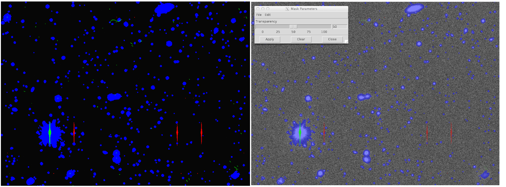
Fig 2. Sky-subtracted data on ds9. Mask image(left), and object image superposed on masked one.

Fig 3. How to adjust parameters of mask image on ds9
Figure 2 shows the result of sky-subtracted image on ds9. On ds9, mask, object, and variance images are superposed and displayed in one window. If you show the object image with a translucent mask, open [Analysis] > [Mask Parameters] at tool bar in ds9 (Fig 3) and set small value in Transparency (Fig 2. right).
The following explains mask images breifly. The pixels flagged as a mask are the ones affected from cosmic rays or overflow by bright star. The footprint pixels are sometimes flagged (Table 3). These flagged pixels are colored corresponding to mask type on ds9. Table 3 shows the correspondence table. For instance, detected objects are blue, overflow from bright star green, and bad pixels red (Fig 2. left).
| Label of flag | Description | Color on ds9 |
|---|---|---|
| BAD | Bad pixel(issued in HSC) | Red |
| CR | Cosmic rays | Magenta |
| CROSSTALK | Crosstalk | |
| EDGE | CCD at the edge | Yellow |
| INTERPOLATED | Pixels having the interporated value derived from surrounding pixels | Green |
| INTRP | Same as INTERPOLATED | |
| SATURATED | Overflow from saturated pixels | Green |
| SAT | Same as SATURATED | |
| SUSPECT | Pixels suspected to be saturation. The non-linearity is not corrected well. | Yellow |
| UNMASKEDNAN | Pixels having NaN value in ISR imageISR | |
| DETECTED | A part of footprint of detected object | Blue |
| DETECTED_NEGATIVE | A part of object footprint which has negative value | Cyan |
| CLIPPED | Pixels clipped in coadd processing (only coadd data) | |
| NO_DATA | Pixels having no input data in coadd processing (only coadd data) |
SourceCatalog
You can search or refer to catalogs created by HSC pipeline using SourceCatalog and butler. In the object catalog, there are object names in columns and mesurements (e.g. flux, position) in rows. The mesurements of ‘float’ or ‘int’ type are extracted by sources.get(” ”). If you extract a certain measurement for all objects, you can use loop processing. Please refer to Contents of SRC-[visit]-[ccd].fits generated after reduceFrames.py or Contents of src-[filter]-[tract]-[patch].fits generated after stack.py for all measurements information.
Two examples, the case of displaying PSF flux in the catalog and the one of magnitude converted from the flux, are shown below.
# Import pythom module
import numpy

""" Search PSF flux """
# Loading SourceCatalog with butler
sour = butler.get("src", dataId)

# Get the number of objects in the catalog
n = len(sources)
n
        # > 1922

# Get PSF flux value
psfflux = sources.get("flux.psf")

# Extract PSF flux for each objects and the value of 'extendedness' from SourceRecord
for i, src in enumerate(sour):
        print i, psfflux[i], src.get("classification.extendedness")

        #(Redults: from left, object number[0-1922], PSF flux, and extendedness)
        # 0 nan 1.0
        # 1 nan 1.0
        # 2 nan 1.0
        # 3 nan 1.0
        #  :
        #  :
        # 1918 600.487226674 1.0
        # 1919 618.323853071 1.0
        # 1920 578.070700843 1.0
        # 1921 nan 1.0


""" Convert PSF flux to magnitude """
# Get information of the origin CCD
metadata = butler.get("calexp_md", dataId)
zeropoint = 2.5 * numpy.log10(metadata.get("FLUXMAG0"))
zeropoint
        # > 30.595966894420105

# Convert PSF flux to magnitude
psfmag = zeropoint - 2.5 * numpy.log10(psfflux)

# Extract derived magnitude from SourceRecord
for i, src in enumerate(sour):
        print i, psfmag[i]

        #(Results: from left, object number[0-1922], PSF flux, and extendedness)
        # 0 nan
        # 1 nan
        # 2 nan
        # 3 nan
        #  :
        #  :
        # 1918 23.6497074602
        # 1919 23.6179268929
        # 1920 23.6910144995
        # 1921 nan
You can make a figure by matplotlib using these measurements results. For example, the frequency distribution of the magnitude derived from PSF flux is checked.
# Import python module
from matplotlib.pyplot import *
from matplotlib.figure import *

# Making frequency distribution of the magnitude and showing it
hist(psfmag, bins=40, range=(10,30))
xlabel('magnitude(PSF)')
show()
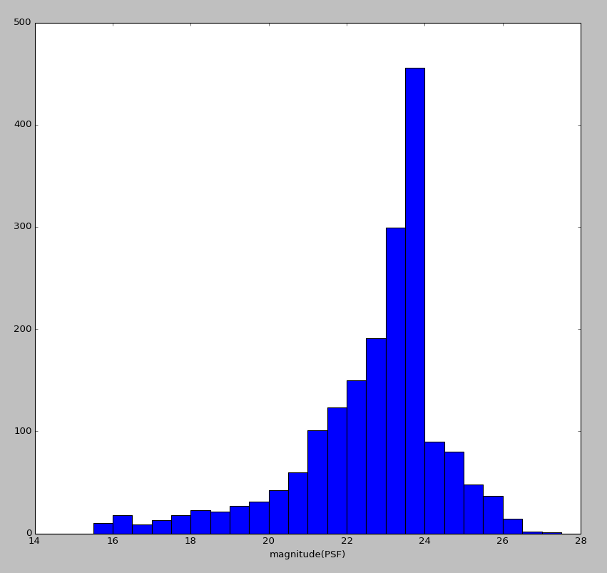
Fig 4. Frequency distribution of the magnitude derived from PSF flux
Next, the ways of checking positional information in the catalog are described. The positional information is stored in a variable, coord. It is a specific data type called Angle, including RA, Dec, and information of coordinate transformation. The coodinate systems are ICRS, FK5, Galactic, and Ecliptic(note that ICRS and FK5 is the same). Degrees, radius, arcminutes, and arcseconds are available as a unit.
Then, let’s check various coordinates in the catalog
# Get coordimate information of all objects in the catalog (ICRS is a basic one)
for src in sour[0:n]:
        icrs      = src.get('coord')
        galactic  = icrs.toGalactic()
        fk5       = icrs.toFk5()
        ecliptic  = icrs.toEcliptic()

        # Get Ra, Dec [deg] in ICRS system
        ra, dec    = icrs.getRa(),         icrs.getDec()

        # Get in other systems
        l, b       = galactic.getL(),      galactic.getB()
        ra2, dec2  = fk5.getRa(),          fk5.getDec()
        lamb, beta = ecliptic.getLambda(), ecliptic.getBeta()
        lon, lat   = icrs.getLongitude(),  icrs.getLatitude()

        sid = src.getId()

        # Display these info on the terminal
        print "ID: ", sid
        print "   ICRS        RA/Dec    (deg)", ra.asDegrees(), dec.asDegrees()
        print "   FK5         RA/Dec    (rad)", ra2.asRadians(), dec2.asRadians()
        print "   Galactic       l/b (arcmin)", l.asArcminutes(), b.asArcminutes()
        print "   Ecliptic lamb/beta (arcsec)", lamb.asArcseconds(), beta.asArcseconds()
        print "   Generic   Long/Lat    (str)", lon, lat


        """ Results
        ID:  775497830381912065
                ICRS        RA/Dec    (deg) 237.77835192 10.1021786534
                FK5         RA/Dec    (rad) 4.15001513096 0.176316279126
                Galactic       l/b (arcmin) 1189.90186102 2667.63454255
                Ecliptic lamb/beta (arcsec) 838482.263154 106153.9408
                Generic   Long/Lat    (str) 4.15002 rad 0.176316 rad
        ID:  775497830381912066
                ICRS        RA/Dec    (deg) 237.778311856 10.0840572239
                FK5         RA/Dec    (rad) 4.15001443172 0.176000000516
                Galactic       l/b (arcmin) 1188.5591858 2667.12102399
                Ecliptic lamb/beta (arcsec) 838500.362538 106090.634831
                Generic   Long/Lat    (str) 4.15001 rad 0.176 rad
         :
         :

        ID:  775497830381913985
                ICRS        RA/Dec    (deg) 237.585304192 10.1094545794
                FK5         RA/Dec    (rad) 4.14664581249 0.176443267991
                Galactic       l/b (arcmin) 1182.84956225 2677.87959672
                Ecliptic lamb/beta (arcsec) 837712.866183 106012.221798
                Generic   Long/Lat    (str) 4.14665 rad 0.176443 rad
        ID:  775497830381913986
                ICRS        RA/Dec    (deg) 237.583434907 10.1064926507
                FK5         RA/Dec    (rad) 4.14661318733 0.176391572584
                Galactic       l/b (arcmin) 1182.55610941 2677.89237965
                Ecliptic lamb/beta (arcsec) 837708.488308 106000.261247
                Generic   Long/Lat    (str) 4.14661 rad 0.176392 rad
        """