Mosaicking
In order to coadd multiple visit images, you have to define the tract and determine wcs and flux scale.
Define tract
We use makeDiscreteSkyMap.py to define tract. Based on the coordinates in the header, the tract is determined as a square covering the entire observed area specified with –id. You have to select all visits and filters for each target (target field) because the tract definition depends on the selected data. In case of the object observed with two filters, if you execute makeDiscreteSkyMap.py to each filter data, the definition of tract/patch can be slightly different. It can cause failures of stack and multi-band analysis.
# Assume that a directory for reduction is ~/HSC, rerun name is test, and field name is test_field (you can check your field name with registry.sqlite3).
makeDiscreteSkyMap.py ~/HSC --calib ~/HSC/CALIB --rerun test --id field=test_field

# makeDiscreteSkyMap.py [data reduction directory] --calib [calib directory] --rerun [rerun name] --id [visit, field, filter..]
# Option
#       --id : Specify all data used to define tract.
You can see the following message when the process is finished successfully.
makeDiscreteSkyMap INFO: tract 0 has corners (177.676, 57.388), (173.867, 57.388), (173.752, 59.440), (177.790, 59.440) (RA, Dec deg) and 11 x 11 patches

# It means that the tract 0 which has 11x11 patch is determined
If you want to define your tract as same as HSC-SSP, use makeSkyMap.py (Defining tract same as SSP).
Mosaicking
Next, you need to match the wcs and flux scale of each visit/CCD data. It can be done by mosaic.py. This command generates a matched list of reference bright stars from each CCD in a given tract. Then it solves spatially-varying correction terms of relative positions and flux scales on different CCDs/visits.
Note
Use either jointcal.py or mosaic.py.
From hscpipe7, mosaic process changes over from mosaic.py to jointcal.py, which is faster than mosaic.py. However, at this point (Nov. 2019), there is a photometric offset (~>5%) among some of the data processed with jointcal.py. We are still solving this problem. Untill the photometric problem is solved, it is safetly to use mosaic.py.
Note that the output files of mosaic.py and jointcal.py are not the same. Then, the files generated by jointcal.py are not removed when you run mosaic.py after jointcal.py. You can see which files are processed by CoaddDriver.py from its output images.
# A directory for reduction is ~/HSC, and rerun name is test
# Execute to each filter
jointcal.py ~/HSC/ --calib ~/HSC/CALIB --rerun test --id visit=20878..20890:2 tract=0 ccd=0..103

# jointcal.py [data reduction directory] --calib [calib directory] --rerun [rerun name] --id [visit, field, filter, ccd] tract=[tract]
# Options
#       --id : Specify the object ID. You can also use field and filter. The tract must be selected here.
#                If you set tracts with makeskyMap.py and do not know the tract ID, run without setting tract.
mosaic.py is used in hscPipe6 or earlier. mosaic.py command is the follows;
# A directory for reduction is ~/HSC, and rerun name is test
# Execute to each filter
# If you get an error like version `GLIBCXX_***' not found in mosaic.py,
# export LD_LIBRARY_PATH=“$LD_LIBRARY_PATH:/work/hscpipe/7.9.1/lib64” etc.
# and add path.
mosaic.py ~/HSC/ --calib ~/HSC/CALIB --rerun test --id visit=20878..20890:2 tract=0 ccd=0..103

# When you output mosaic validation in ~/HSC/rerun/mosaic_diag,
mosaic.py ~/HSC/ --calib ~/HSC/CALIB --rerun test --id visit=20878..20890:2 tract=0 ccd=0..103 --diagnostics --diagDir ~/HSC/rerun/mosaic_diag

# mosaic.py [data reduction directory] --calib [calib directory] --rerun [rerun name] --id [visit, field, filter, ccd] tract=[tract]
# Options
#       --id : Specify the object ID. You can also use field and filter. The tract must be selected here.
#       --diagnostics : Add this options if you want to output the results of validation.
#       --diagDir : Specify a output directory for validation.
Note
Depending on your machine environment, it takes over 30 minutes after the following messages;
Mosaic INFO: Reading catalogs…
Mosaic INFO: Use 1 cores for reading source catalog
After mosaicking is completed, you find flux scaling files jointcal_photoCalib-[visit]-[ccd].fits and corrected wcs files jointcal_wcs-[visit]-[ccd].fits in ~/HSC/rerun/[rerun]/jointcal-results/[tract]. They are the flux scale and wcs coordinate transformation files for each visit and CCD.
If you add option –diagnostics, you also find the following validation result files in the directory specified by –diagDir.
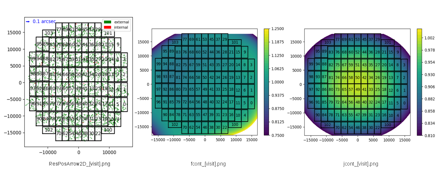
Validation results in each visit
Positional offsets : ResPosArrow2D_[visit].png
Residuals of flux to distortion pattern: fcont_[visit].png
Distortion pattern of reduceFlat : jcont_[visit].png(confirm that distributions is in a concentric fashion)
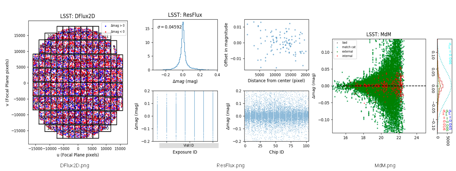
Validation results in all visit
Deviation from mean flux of each visit : DFlux2D.png
Residuals of fluxes : ResFlux.png
Deviation in magnitudes of detected sources (※): MdM.png
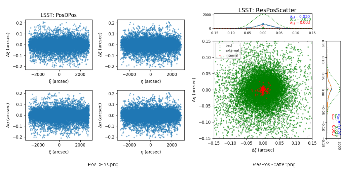
Offsets of WCS : PosDPos.png
Offsets of WCS : ResPosScatter.png
- Other outputs
catalog.fits
ccd.dat
ccdScale.dat
coeffs.dat
dmag.dat
dpos.dat
(※) MdM.png & ResPosScatter.png; Green points show deviation of catalogs in HSC pipeline from astrometry catalog while red points show deviation from the mean of all visit in sources which are not in MATCH catalog.
Applying the mosaic solution to each visit/CCD data
Then apply the wcs and flux scale determined by mosaic.py to each visit/CCD data.
Note
Currently (Nov. 2019), there are some defects in outputs of calibrateExposure.py and calibrateCatalog.py . If you want to see each CCD and catalog precisely, do this step just after mosaic.py. Otherwise do this step at the end of all processing. If you do not need to calibrate wcs and zero-point, you don’t need this step.
Use calibrateExposure.py to apply the solution found with mosaic.py to CORR images.
# Applying the solution to the visit/CCD images
# Directory for reduction is ~/HSC, and rerun name is test
calibrateExposure.py ~/HSC --calib ~HSC/CALIB --rerun test --id field=NGC604 tract=0 ccd=0..103 -j 8

# calibrateExposure.py [data reduction directory] --calib [calib directory]  --rerun [rerun name] --id [field, tract, ccd] -j [the number of threads]
# Options
#       --id : In the example, the input data is selected as a combination of field, tract and ccd. You can also use the combination of visit and ccd.
#       -j : Specify the number of threads.
Then you find calibrated images named ~/HSC/rerun/[rerun]/[pointing]/[filter]/corr/[tract]/CALEXP-[visit]-[ccd].fits
Use calibrateCatalog.py to apply the mosaic.py’s solution to SRC catalogs.
# Applying the solution to catalogs.
# Directory for reduction is ~/HSC, and rerun name is test
calibrateCatalog.py ~/HSC --calib ~/HSC/CALIB --rerun test --id field=NGC604 tract=0 ccd=0..103 --config doApplyCalib=False -j 8

# calibrateCatalog.py [data reduction directory] --calib [calib directory] --rerun [rerun name] --id [field, tract, ccd] -j [the number of threads]
# Options
#       --id : Same as calibrateExposure.py, you can also use the combination of visit and ccd.
#       --config doApplyCalib=False : Add it if you do not calibrate fluxes to magnitudes.
#       -j : Specify the number of threads.
The calibrated catalogs are ~/HSC/rerun/[rerun]/[pointing]/[filter]/output/[tract]/CALSRC-[visit]-[ccd].fits.